Research
Major Research Result
Major Research Result of the Korea Ocean Satellite Center
-
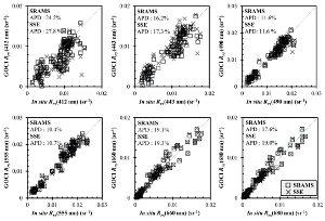
An estimation of the aerosol multiple-scattering reflectance is an important part of the atmospheric correction procedure in satellite ocean color data processing. Most commonly, the utilization of two near-infrared (NIR) bands to estimate the aerosol optical properties has been adopted for the estimation of the effects of aerosols. Previously, the operational Geostationary Color Ocean Imager (GOCI) atmospheric correction scheme relies on a single-scattering reflectance ratio (SSE), which was developed for the processing of the Sea-viewing Wide Field-of-view Sensor (SeaWiFS) data to determine the appropriate aerosol models and their aerosol optical thicknesses. The scheme computes reflectance contributions (weighting factor) of candidate aerosol models in a single scattering domain then spectrally extrapolates the single-scattering aerosol reflectance from NIR to visible (VIS) bands using the SSE. However, it directly applies the weight value to all wavelengths in a multiple- scattering domain although the multiple-scattering aerosol reflectance has a non-linear relationship with the single-scattering reflectance and inter-band relationship of multiple scattering aerosol reflectances is non-linear. To avoid these issues, we propose an alternative scheme for estimating the aerosol reflectance that uses the spectral relationships in the aerosol multiple-scattering reflectance between different wavelengths (called SRAMS). The process directly calculates the multiple-scattering reflectance contributions in NIR with no residual errors for selected aerosol models. Then it spectrally extrapolates the reflectance contribution from NIR to visible bands for each selected model using the SRAMS. To assess the performance of the algorithm regarding the errors in the water reflectance at the surface or remote-sensing reflectance retrieval, we compared the SRAMS atmospheric correction results with the SSE atmospheric correction using both simulations and in situ match-ups with the GOCI data. From simulations, the mean errors for bands from 412 to 555 nm were 5.2% for the SRAMS scheme and 11.5% for SSE scheme in case-I waters. From in situ match-ups, 16.5% for the SRAMS scheme and 17.6% scheme for the SSE scheme in both case-I and case-II waters. Although we applied the SRAMS algorithm to the GOCI, it can be applied to other ocean color sensors which have two NIR wavelengths.
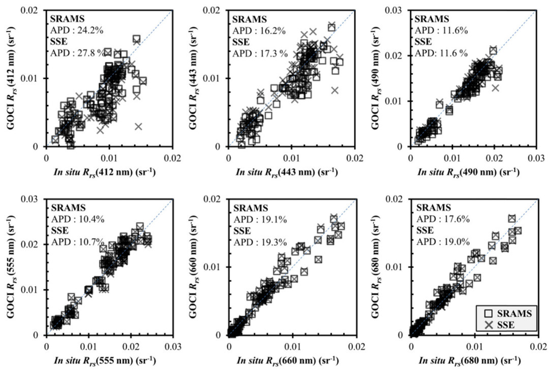
Figure. Validation results of in situ Rrs match-ups at different visible wavelengths of GOCI, 412, 443, 490, 555, and 660 nm for SRAMS and SSE scheme. In situ Rrs data are from Korea Ocean Satellite Center (KOSC) cruises since 2010 (65 match-ups) and the ocean color component of the Aerosol Robotics Network (AERONET-OC) sites (67 match-ups).
-
Estimation ofchlorophyll concentration in themarine biosphere has been the central topic ofocean color remote sensing since its advent. While various algorithms were proposed in the literature so far and tested for oceanic waters ofdiverse constituent composition, an independent algorithmevaluation is needed for local oceanwaters that have dynamic variation in optically active water constituents such as colored dissolved organic matters (CDOM) and suspended particulate matter (SPM). This paper evaluates the performance of chlorophyll algo- rithms for Geostationary Ocean Color Imager (GOCI) radiometric data, using in situ measurements collected at 491 stations around Korea Peninsula during 2010–2014 from which there were 130 match-ups with GOCI data. For the evaluation in areas with high variation in SPM, water samples were first classified into three levels ofSPM, and then the coefficients of candidate algorithms were newly derived for the turbidity cases using the in situ and GOCI remote sensing reflectance (Rrs) data. Functional forms of traditional band ratio algorithms (e.g. OC algorithms (O′Reilly et al., 1998) and Tassan's algorithm (Tassan, 1994)), fluorescence line height algorithm, and near-infrared-to-red band ratio approachwere tested. The evaluation results for the coincident in situ pairs ofRrs and chlorophyll measurements showed that the mean uncertainty was b35% with the correlation around 0.8 by using the OC3 with turbidity consideration (OCT) and Tassan's algorithm with turbidity dependent coefficients (Tassan-TD). For the GOCI match-ups, themean uncertainty for all turbidity levels was around 35%with correla- tion around 0.65, when OCT and Tassan-TD were used.
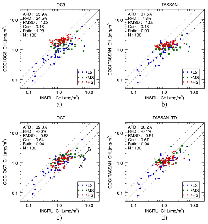
Figure. Scatter plots between the in situ CHL and the CHL estimated fromGOCI Rrs are presented for (a) OC3, (b) Tassan, (c) OCT, and (d) Tassan-TD. Statistics presented in the figures are for all samples.
-
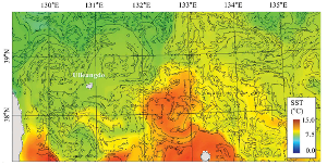
We attempted for the first time to extract fronts from ocean colour data acquired at a geostationary orbit derived from the Geostationary Ocean Color Imager (GOCI), the world’s first geostationary ocean colour satellite sensor. We extracted fronts from hourly observed GOCI images and then attempted to investigate subtle changes in ocean condition. Suspended sediment (SS)-derived fronts were used to analyse tidal movements in a coastal region having semi-diurnal tides and highly turbid water. We were able to trace fast movements of tidal flows and discovered that the SS-derived ocean fronts are quite relevant to the submarine topography along shallow coasts. In relatively clear waters using chlorophyll concentration (chl)-derived fronts,wewereabletodiscoverdynamic variations on sea areas where two independent water masses mixed. We also found that GOCI-derived fronts can provide more detailed information than can SST-derived fronts. We expect that such results can be utilized to search for productive fisheries
Figure. GOCI chl-derived front map (black lines) at 12:30 compared with daily SST data distribution (coloured image) around the JES on 5 April 2011. The the East Korea Warm Current (EKWC) and the North Korea Cold Current (NKCC) meet at about 38°N, forming the polar frontal zone in the centre of the JES and facilitating oceanic eddies around Ulleungdo.
-
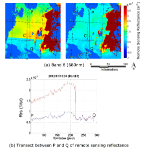
The Geostationary Ocean Color Imager (GOCI) is the world’s first ocean color sensor in geostationary orbit. Although the GOCI has shown excellent radiometric performance with little long-term radiometric degradation and a high signal-to-noise ratio, there are radiometric artefacts in GOCI Level 1 products caused by stray light detected within the GOCI optics. To correct the radiometric bias, we developed an image-based correction algorithm called the correction of the interslot discrepancy using the minimum noise fraction transform (CIDUM) in a previous study and evaluated its performance with respect to the physical radiometric quantity stored in Level 1 products, i.e., top-of-atmosphere radiance. This study evaluated the performance of the CIDUM algorithm in terms of remote sensing reflectance, which is one of the most important products in ocean color remote sensing. The resultant CIDUM-corrected remote sensing reflectance products were validated using both relative (within the image) and absolute references (in situ measurements). Image validation showed that CIDUM corrected the bias in remote sensing reflectance (up to 20%) and reduced the bias to ?5% in the tested image. In situ validation showed that relative uncertainty was reduced by around 10% within the visible bands and the correlation between the in situ and GOCI radiometric data was enhanced.

Figure. (a) Images of GOCI remote sensing reflectance acquired on 16 October 2012 (UTC 04) for Band 6 both before and after the CIDUM correction; (b) Profile of remote sensing reflectance along transect PQ.
-
This paper reanalyzes the aerosol reflectance correction schemes employed by major ocean color missions. The utilization of two near-infrared (NIR) bands to estimate aerosol reflectance in visible wavelengths has been widely adopted, for example by SeaWiFS/MODIS/VIIRS (GW1994), OCTS/GLI/SGLI (F1998), MERIS/OLCI (AM1999), and GOCI/GOCI-II (A2016). The F1998, AM1999, and A2016 schemes were developed based on GW1994; however, they are implemented differently in terms of aerosol model selection and weighting factor computation. The F1998 scheme determines the contribution of the most appropriate aerosol models in the aerosol optical thickness domain, whereas the GW1994 scheme focuses on single-scattering reflectance. The AM1999 and A2016 schemes both directly resolve the multiple scattering domain contribution. However, A2016 also considers the spectrally dependent weighting factor, whereas AM1999 calculates the spectrally invariant weighting factor. Additionally, ocean color measurements on a geostationary platform, such as GOCI, require more accurate aerosol correction schemes because the measurements are made over a large range of solar zenith angles which causes diurnal instabilities in the atmospheric correction. Herein, the four correction schemes were tested with simulated top-of-atmosphere radiances generated by radiative transfer simulations for three aerosol models. For comparison, look-up tables and test data were generated using the same radiative transfer simulation code. All schemes showed acceptable accuracy, with less than 10% median error in water reflectance retrieval at 443 nm. Notably, the accuracy of the A2016 scheme was similar among different aerosol models, whereas the other schemes tended to provide better accuracy with coarse aerosol models than the fine aerosol models.
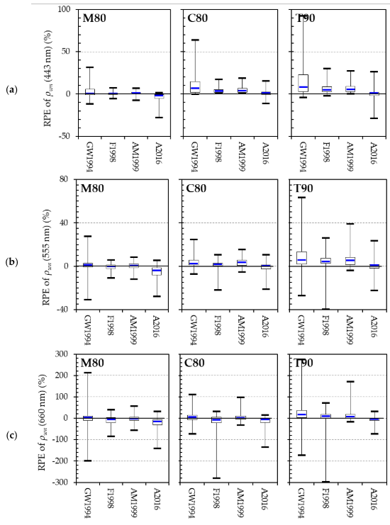
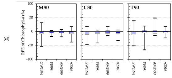
Figure. Water reflectance (ρwn) retrieval accuracy of the (a) blue; (b) green; and (c) red bands in the atmospheric correction algorithm after integrating the four aerosol correction schemes. Chlorophyll-a estimation error based on OC3 [33] is plotted in (d).
-

Tidal flats are associated with complicated depositional and ecological environments, and have changed considerably as a result of the erosion and sedimentation caused by tidal energy; consequently, the surface sediment distribution in tidal flats must be constantly monitored and mapped. Although several studies have been conducted with the aim of classifying intertidal surface sediments using various remote sensing methods combined with field survey, most of these studies were unable to consider various sediment types, due to the low spatial resolution of remotely sensed data. Therefore, previous studies were unable to efficiently describe precise surface sediment distribution maps. In the present study, unmanned aerial vehicle (UAV) red, green, blue (RGB) orthoimagery was used in combination with a field survey (232 samples) to produce a large-scale classification map for surface sediment distribution, in accordance with sedimentology standards, using an object-based method. The object-based method is an effective technique that can classify surface sediment distribution by analyzing its correlations with spectral reflectance, grain size, and tidal channels. Therefore, we distinguished six sediment types based on their spectral reflectance and sediment properties, such as grain composition and statistical parameters. The accuracy assessment of the surface sediment classification based on these six types indicated an overall accuracy of 72.8%, with a kappa coefficient of 0.62 and 5-m error range related to the Global Positioning System (GPS) device. We found that 11 samples were misclassified due to the effects of sun glint and cloud caused by the UAV system and shellfish beds, while 14 misclassified samples were influenced by surface water related to the elevation, tidal channels, and sediment properties. These results indicate that large-scale classification of surface sediment with high accuracy is possible using UAV RGB orthoimagery.
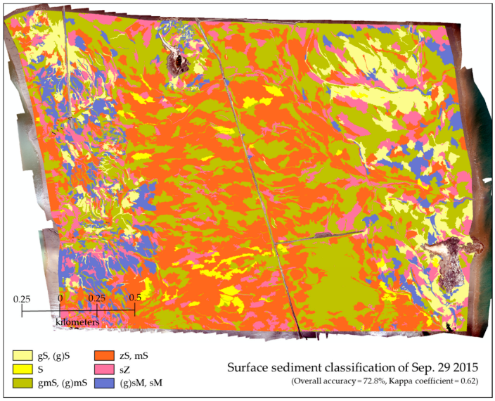
Figure. Large-scale surface sediment classification map derived from the UAV RGB orthoimage. The overall accuracy is 72.8%, with a 5-m error range, and the Kappa coefficient is 0.62.
-
Since 2008, floating green tides (Ulva sp.) have been occurring continuously in the Yellow Sea (YS), and after 2013 floating golden tides (Sargassum sp.) have also occurred. The distribution, areal coverage, and migration of floating green tides have been actively studied, but most research has focused only on the western YS. Little is known about the floating golden tides in the eastern YS. The purpose of this study was to determine the long-term distribution of floating green and golden tides in the eastern YS using Geostationary Ocean Color Imager (GOCI), Moderate Resolution Imaging Spectroradiometer (MODIS), and Landsat satellite images from 2008 to 2017. In addition, the migration of floating macroalgae with Global Hybrid Coordinate Ocean Model (HYCOM) surface current data were compared. Green tides were observed in 2008, 2009, 2011, 2015, and 2016 in the eastern YS. From a satellite image backtracking analysis, it was confirmed that the green tides observed in the eastern YS were supplied from the western YS. When the maximum areal coverage of green tide was compared between the eastern and western YS, the coverage in the eastern YS was found to be about 4 % of that of the western YS. However, in 2011, the largest amount of floating macroalgae was found in the eastern YS and it accounted for about 45 % of the amount in the western part of the YS. In the eastern YS, floating golden tides were found in 2013, 2015, 2016, and 2017, with the largest amount of floating macroalgae occurring in 2017. Although there were no long-term golden tide data for the western YS, such that it was not compared to the areal coverage of the eastern YS, it was confirmed that the amount of golden tide supplied to the eastern YS gradually increased. A comparison between the migration of floating macroalgae and HYCOM surface current data suggested that the migration and flow directions were not identical, and were considerably affected by surface ocean currents during their passage into the eastern YS. From this study, the long-term distribution and changes in areal coverage of green and golden tides in the eastern YS were obtained for the first time. This information will be useful for understanding the long-term patterns of green and golden tides, and provides basic data for predicting the occurrence and migration of floating macroalgae.

Figure1. Long-term trend of green tides in the eastern YS.
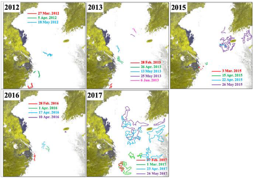
Figure2. Long-term trend of golden tides in the eastern YS. -
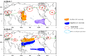
We show two major modes of East Asian marine heatwaves (MHWs) associated with two contrasting sea surface temperature patterns over the subtropical western North Pacific (WNP). In the first MHW mode, ocean warming over East Asia occurs along with the subtropical WNP from the earlier winter by an El Niño-Southern Oscillation. The basin-wide ocean warming is finally intensified to an extreme warming state around East Asia, where a high-pressure region in zonal waves across the Eurasian continent passes. In contrast, at the early stage, the second MHW mode is unfavorable with ocean cooling. However, MHWs over East Asia occur due to a significant intensification of a zonally elongated high-pressure zone in response to anomalous subtropical convection in addition to mid-latitude zonal waves. Due to the importance of persistent ocean warming as well as immediate atmospheric forcing, MHW inducible oceanic and atmospheric interactions are clearly distinguishable from those of atmospheric heatwaves.
Figure. Schematic pictures illustrating how two primary modes of East Asian marine heatwaves are affected by global-scale climate variabilities (CGT, WNP convection, and the equatorial SST pattern): (a) Mode 1 (basin-wide warming pattern) and (b) Mode 2 (dipole warming pattern).
-
Geostationary Ocean Color Imager (GOCI) observations are applied to marine fog (MF) detection in combination with Himawari-8 data based on the decision tree (DT) approach. Training and validation of the DT algorithm were conducted using match-ups between satellite observations and in situ visibility data for three Korean islands. Training using different sets of two satellite variables for fog and nonfog in 2016 finally results in an optimal algorithm that primarily uses the GOCI 412-nm Rayleigh-corrected reflectance (Rrc) and its spatial variability index. The algorithm suitably reflects the optical properties of fog by adopting lower Rrc and spatial variability levels, which results in a clear distinction from clouds. Then, cloud removal and fog edge detection in combination with Himawari-8 data enhance the performance of the algorithm, increasing the hit rate (HR) of 0.66 to 1.00 and slightly decreasing the false alarm rate (FAR) of 0.33 to 0.31 for the cloudless samples among the 2017 validation cases. Further evaluation of Cloud-Aerosol Lidar and Infrared Pathfinder Satellite Observation data reveals the reliability of the GOCI MF algorithm under optically complex atmospheric conditions for classifying marine fog. Currently, the high-resolution (500 m) GOCI MF product is provided to decision-makers in governments and the public sector, which is beneficial to marine traffic management.
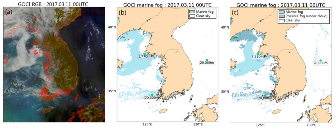
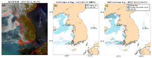
Figure. (a) GOCI RGB image and marine fog detection image obtained from the GOCI marine fog detection algorithm (b) without and (c) with postprocessing on 2017.03.11 at 00 UTC. The white and sky-blue areas indicate clear-sky sea and marine fog regions, respectively, and the gray area is the region with clouds or marine fog under clouds. The numbers below the marks are the observed visibility at each station. In addition, the color of the filled circle at the stations is red with a visibility less than 1 km, but green with a visibility greater than 1 km.
-
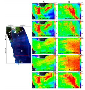
The red tide bloom-forming dinoflagellate Margalefidinium polykrikoides is well known for its harmful effects on marine organisms, and for killing fish in aquaculture cages via gill clogging at a high cell abundance. To minimize the damage caused by red tide blooms, it is essential to understand their detailed spatial distribution with high accuracy. Airborne hyperspectral imagery (HSI) is useful for quantifying red tide cell abundance because it provides substantial information on optical features related to red tide species. However, because published red tide indexes were developed for multichannel ocean color sensors, there are some limitations to applying them directly to HSI. In this study, we propose a new index for quantifying M. polykrikoides blooms along the south coast of Korea and generate a M. polykrikoides cell abundance map using HSI. A new index for estimating cell abundance was proposed using the pairs of M. polykrikoides cell abundances and in situ spectra. After optimization of the published red tide indexes and band correlation analyses, the green-to-fluorescence ratio (GFR) index was proposed based on red tide spectral characteristics. The GFR index was computed from the green (524 and 583 nm) and fluorescence wavelength bands (666 and 698 nm) and converted into red tide cell abundance using a second-order polynomial regression model. The newly proposed GFR index showed the best performance, with a coefficient of determination (R2) of 0.52, root mean squared error (RMSE) of 877.98 cells mL−1, and mean bias error (MBE) of −18.42 cells mL−1, when applied to atmospherically corrected HSI. The M. polykrikoides cell abundance map generated from the GFR index provides precise spatial distribution information and allowed us to estimate a wide range of cell abundance up to 5000 cells mL−1. This study indicates the potential of the GFR index for quantifying M. polykrikoides cell abundance from HSI with a reasonably high level of accuracy.
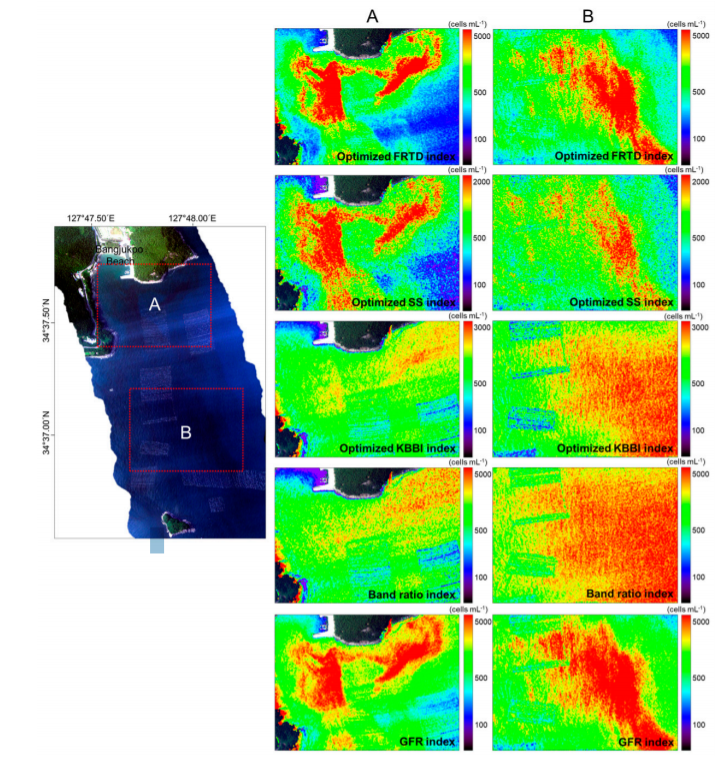
Figure. HSI true-color composite image (R, 639.52 nm; G, 550.58 nm; B, 469.92 nm) and M. polykrikoides cell abundance maps near Bangjukpo Beach in Yeosu on 8 August 2018. Sections (A) and (B) in the HIS image are enlarged on the right panels. M. polykrikoides cell abundance maps were generated using optimized red tide indexes, the band ratio index, and the GFR index